Facing the SnowStorm: Part 2

Recap from Part 1

Welcome back! In part 1 of this two-part series on Snowflake Query Performance, we learned that simply upping the size of our Snowflake virtual warehouse didn’t do much for improving query performance. So, if it's not compute power, what's going on? The issue might actually lie in how the data is structured. In this part, we’re going to dig into clustering and partitioning to see if these could be the missing pieces to the puzzle. Let's see if we can finally get to the bottom of this.

Snowflake Micro-Partitions and Data-Clustering

Micro-partitions

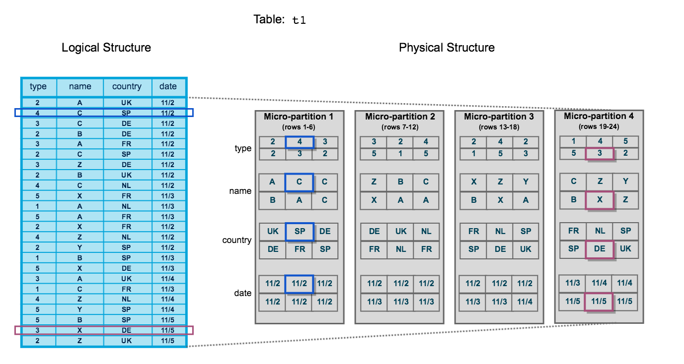
All data in Snowflake tables is automatically divided into micro-partitions, which are contiguous units of storage. Groups of rows in tables are mapped into individual micro-partitions, organized in a columnar fashion. This size and structure allows for extremely granular pruning of very large tables, which can be comprised of millions, or even hundreds of millions, of micro-partitions. Snowflake stores metadata about all rows stored in a micropartition, including:

- The range of values for each of the columns in the micro-partition.

- The number of distinct values.

- Additional properties used for both optimization and efficient query processing.

According to Snowflake, these micropartitions are applied automatically to any data inserted into any table, and is primarily used for the goal of Query Pruning.

The micro-partition metadata maintained by Snowflake enables precise pruning of columns in micro-partitions at query run-time, including columns containing semi-structured data. In other words, a query that specifies a filter predicate on a range of values that accesses 10% of the values in the range should ideally only scan 10% of the micro-partitions.

Rabbit Hole Interlude: Partitions vs Indexes

Snowflake's concept of micro-partitions (let's just call them 'partitions') and the index of most traditional Relational Database Management Systems (RDBMS) serve different but complementary purposes in that they both handle data access patterns.

Partitions in Snowflake use a columnar storage format, and play a huge role in how Snowflake optimizes its underlying data storage and retrieval. Think of them as physical chunks of data allocated together (or closeby) on a disk. Snowflake also keeps metadata about which data is stored in each partition (think of it like a directory of physical stores in a shopping center). This metadata is part of the partition and is stored alongside the actual data.

This helps the Snowflake Query Optimizer with data pruning, aka deciding which parts of a disk are irrelevant to the query it's looking to run based on the metadata (directory) that it knows about each partition. Suppose if you have a WHERE clause that specifies a particular CUSTOMER_ID, all the query optimizer has to do is go to the location on disk that has that particular CUSTOMER_ID as a key, therefore discarding all the other partitions that are irrelevant to its query. This is an oversimplification, which we'll discuss a bit later when we talk about data-clustering.

Similarly in theme (but not in implementation), indexes in MySQL are mainly used to speed up the retrieval or rows from a table. Think of a data structure that exists separately from the actual table data (typically a B-Tree) that stores the values for a particular column (or group of columns). The query optimizer can therefore quickly locate the data without having to scan every single row in a table.

So while both approaches serve the same purpose of speeding up queries by eliminating irrelevant pieces of the data, they go about things quite differently. To remember is that Snowflake's partitions are designed to scan huge amounts of data quickly (across different datasets even), while indexes are much smaller in scope and are usually restricted to a single table.

Data Clustering

In addition to micro-partitions, Snowflake further organizes data in data-clusters

Typically, data stored in tables is sorted/ordered along natural dimensions (e.g. date and/or geographic regions). This “clustering” is a key factor in queries because table data that is not sorted or is only partially sorted may impact query performance, particularly on very large tables.

In Snowflake, as data is inserted/loaded into a table, clustering metadata is collected and recorded for each micro-partition created during the process. Snowflake then leverages this clustering information to avoid unnecessary scanning of micro-partitions during querying, significantly accelerating the performance of queries that reference these columns.

As an analogy, a cluster is a directory of directories (partitions) that allows the Query Optimizer to do an initial pruning of all the micro-partitions it knows about. More information here

Interlude: Clustering Keys

Before we dive in further, I should briefly mention Clustering Keys.

As a table grows in size, the data in some table rows might no longer cluster optimally on desired dimensions.
In order to improve the clustering of your table, you can designate one or more columns as the clustering key for your table, which can help improve the clustering of your underlying table micro-partitions. Since you, the developer, (hopefully) understand the access and query patterns in your data a lot better than the query optimizer, you can use clustering keys to provide Snowflake with hints on how to best organize your data.

This excellent article by Harry Tan does a wonderful job further explaining some of these concepts.

A core design principle of Snowflake is to store metadata alongside its tables for fast lookups. So it is with data clusters. The key metric we're interested in for our problem is Clustering Depth.

We're about to do a deep-dive here, so strap in and hold on to your butts.

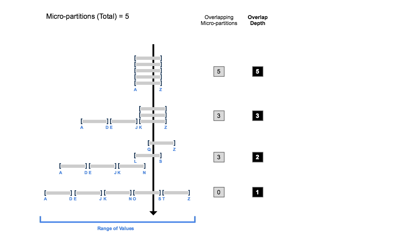
According to Snowflake: The clustering depth for a populated table measures the average depth (1 or greater) of the overlapping micro-partitions for specified columns in a table. The smaller the average depth, the better clustered the table is with regards to the specified columns.

Because multiple micro-partitions can store different types of metadata about the same row or record in a table, there is a potential for overlap between two or more partitions. This means the Query Optimizer needs to check multiple partitions when planning a query, increasing its planning (Snowflake calls this compilation, a remnant from the early Oracle days from its founders) latency. We can reduce this overlap by analysing the clustering depth of a table.

- In the beginning, the range of values in all the micro-partitions overlap.

- As the number of overlapping micro-partitions decreases, the overlap depth decreases.

- When there is no overlap in the range of values across all micro-partitions, the micro-partitions are considered to be in a constant state (i.e. they cannot be improved by clustering).

So, to put in terms our dear friend Grug Developer would be happy with:

1. Partitions good.
2. Clusters also good. Clusters contain partition data. This moar good.
3. Small Clustering Depth Number > Large Clustering Depth Number
4. Moar black think juice (aka coffee) equals moar thinking power.

We can conclude that our slow query performance must be related to these partitions and clustering. However, Snowflake's SnowSight UI does not offer any dashboards or metrics that can tell us more.

We dig deeper to find that Snowflake does expose us some useful information in the form of SYSTEM$CLUSTERING_INFORMATION call.

Given that most of our data lives in the ORDERS_FINAL table, let's focus our efforts here. We run a query on the metadata Snowflake has on our table and look at the results.

select system$CLUSTERING_INFORMATION('ORDERS_FINAL');

 1{
 2  "cluster_by_keys" : "CUSTOMER_ID"
 3  "notes" : "Clustering key columns contain high cardinality key CUSTOMER_ID which might result in expensive re-clustering. Consider reducing the cardinality of clustering keys. Please refer to https://docs.snowflake.net/manuals/user-guide/tables-clustering-keys.html for more information.",
 4  "total_partition_count" : 60,
 5  "total_constant_partition_count" : 12,
 6  "average_overlaps" : 40.2857,
 7  "average_depth" : 27.1429,
 8  "partition_depth_histogram" : {
 9    "00000" : 0,
10    "00001" : 2,
11    "00002" : 2,
12    "00003" : 0,
13    "00004" : 0,
14    "00005" : 5,
15    "00006" : 0,
16    "00007" : 16,
17    "00008" : 8,
18    "00009" : 0,
19    "00010" : 12,
20    "00011" : 0,
21    "00012" : 0,
22    "00013" : 23,
23    "00014" : 0,
24    "00015" : 0,
25    "00016" : 21
26  },
27  "clustering_errors" : [ ]
28}

Disclaimer: For illustration purposes only. Yes, I made up these numbers to prove a point lol.

Let's explain some of these concepts:

CLUSTER_BY_KEYS

Indicates that the table is clustered by the CUSTOMER_ID field, so Snowflake uses this field to organize the data across micro-partitions.

NOTES

The notes mention that the clustering key (BUSINESS_UUID) has high cardinality, which could lead to expensive re-clustering operations. High cardinality means the column has a large number of unique values, which can result in a broad spread of data across many micro-partitions, potentially reducing the effectiveness of clustering (granted, this is less likely for an INT data type, but you get the idea)

TOTAL_PARTITION_COUNT

The total number of micro-partitions in the table is 60. This indicates how the data is divided at the storage level.

TOTAL_CONSTANT_PARTITION_COUNT

Out of 60 partitions, only 12 are constant. Constant means that these partitions do not overlap with others based on the clustering key. This is typically a bad sign, suggesting that most of the data is poorly-clustered.

AVERAGE_OVERLAPS AND AVERAGE_DEPTH

These metrics show that on average, partitions overlap with about 40 other partitions Additionally, the average depth of these overlaps is around 27. This suggests severe overlapping and depth, indicating that re-clustering could be beneficial especially for those partitions that significantly deviate from this average.

PARTITION_DEPTH_HISTOGRAM

This histogram indicates that most partitions have at least some depth, which is not great. This likely means that the data is too spread out in most partitions.

It looks like our partitioning on the ORDERS_FINAL_TABLE (our fact table) is less than optimal, which could be a possible explanation for our slow queries. We can also run this for every single one of our tables by cobbling together a quick script using the SnowPark API.

 1from itertools import permutations
 2import ast
 3
 4import snowflake.snowpark as snowpark
 5from snowflake.snowpark.functions import col
 6
 7TABLES = ["ORDERS_FACT_FINAL", "CUSTOMER_DIMENSION", "SHIPPING_DIMENSION", # rest of tables... ]
 8
 9def main(session: snowpark.Session):
10    def get_clustering_info(table_name):
11        query = f"SELECT SYSTEM$CLUSTERING_INFORMATION('{table_name}')"
12        print(f"Executing query: {query}")
13        result = session.sql(query).collect()
14        clustering_info = ast.literal_eval(result[0][0])
15
16        print(clustering_info)
17
18        total_partition_count = clustering_info.get("total_partition_count", 0) or 1  # prevent div by zero error
19        total_constant_partition_count = clustering_info.get("total_constant_partition_count", 0) or 1  # prevent div by zero error
20
21        average_depth = clustering_info.get("average_depth", 0)
22        average_overlaps = clustering_info.get("average_overlaps", 0)
23
24        return {
25            "table_name": table_name,
26            "total_partition_count": total_partition_count,
27            "total_constant_partition_count": total_constant_partition_count,
28            "clustering_depth": average_depth,
29            "clustering_depth_percentage": (average_depth / total_partition_count) * 100,
30            "clustering_overlap": average_overlaps,
31            "clustering_overlap_percentage": (average_overlaps / total_partition_count) * 100,
32            "partition_depth_histogram": clustering_info.get("partition_depth_histogram")
33        }
34    clustering_results = [get_clustering_info(table_name) for table_name in TABLES]
35
36    results_df = session.create_dataframe(clustering_results)
37    results_df.sort(col('total_partition_count').asc(), col('clustering_depth_percentage').asc())
38    results_df.show()
39    return results_df
40
41"""
42    TOTAL PARTITION COUNT: 
43    Number of micro-partitions in the table. Higher count means a more fragmented table
44
45    TOTAL_CONSTANT_PARTITION_COUNT:
46    Total number of micro-partitions for which the value of the specified columns 
47    have reached a constant state (i.e. the micro-partitions will not benefit 
48    significantly from reclustering). The number of constant micro-partitions in a 
49    table has an impact on pruning for queries. The higher the number, the more 
50    micro-partitions can be pruned from queries executed on the table, which has a 
51    corresponding impact on performance.
52
53    CLUSTERING DEPTH AVG:
54    Micro-partitions scanned per key range Lower = better clustering
55
56    CLUSTERING DEPTH:
57    (DEPTH / TOTAL PARTITIONS) * 100. A lower percentage == efficient clustering
58
59    CLUSTERING OVERLAP AVG:
60    Overlapping micro-partitions per key range. A lower number == less redundancy
61
62    CLUSTERING OVERLAP:
63    (OVERLAP / TOTAL PARTITIONS) * 100. A lower percentage == efficient storage
64
65    PARTITION DEPTH HISTOGRAM:
66    Distribution of micro-partitions across depth levels, 
67    providing a visual clustering assessment
68"""

It looks like most of our tables are well partitioned, with the exception of our ORDERS_FINAL table.

Given that this is our main FACT table, we're pretty confident at this point that this is our bottleneck.

While we can tell that the partitioning on this table is bad, we still don't know WHY.

After sufficient place-forehead-on-desk-at-high-velocity (aka bang head on desk), we decided to ask the good folks at Snowflake, who were awesome enough to let us sit down with their Field CTO team and have us barrage them with the laundry list of questions we gathered after trying to reverse engineer some of the mechanics of their platform.

Snowflake Micro-Partitions: The Plot Thickens

With the help of the Snowflake Field CTO team, we investigated the partitioning on our tables. Using some internal tooling, the Snowflake team was quickly able to find that our tables were adding more and more micro-partitions by the minute! Y Tho?

The answer: because micro-partitions are immutable. The immutable nature of micro-partitions allows for the lookup and usage of said partitions to be MUCH more performant at query-time. But the flipside of this performance is that, whenever data gets updated or deleted, Snowflake will add new micro-partitions instead of modifying existing ones.

To offset inefficiencies caused by this immutability (and thus the need to create new partitions), Snowflake also has periodic asynchronous automatic re-clustering tasks running in the background, which reorganizes the data across its different nodes and helps the queries remain performant.

This is further confirmed by this Snowflake Blog article from May 2022:

Snowflake micro-partitions immutable files that are not visible to the Snowflake user; rather, the table acts as a container of micro-partitions and that is what the user will interact with. Some of the interactions are:

- A SQL INSERT operation that will load new records as new micro-partitions....

Looking back at our initial ingestion architecture, which component makes continuous updates to the tables? Right, THE TRIGGERED TASK.

Triggered Task == VILLAIN?

Let's look again at our triggered task definition:

 1-- ...
 2as MERGE INTO ORDERS_FINAL USING (
 3                    SELECT *
 4     FROM ORDERS_STAGING_STREAM
 5     QUALIFY ROW_NUMBER() OVER ( -- this QUALIFY statement is important - see below.
 6      PARTITION BY CUSTOMER_ID, ORDER_ID
 7      ORDER BY CREATED_AT DESC
 8     ) = 1
 9    ) AS STG_STREAM ON ORDERS_FINAL.CUSTOMER_ID = STG_STREAM.CUSTOMER_ID
10    AND ORDERS_FINAL.ORDER_ID = STG_STREAM.ORDER_ID
11    WHEN MATCHED THEN
12    UPDATE -- If relevant records are found in ORDERS_FINAL, update values with the stream's values, as we know that's the latest version of the record
13    SET
14     ORDERS_FINAL.RECORD_UUID = STG_STREAM.RECORD_UUID,
15-- ...

We know that this task runs each time it detects new data in the stream it's "listening" to. If the ORDERS_STAGING_STREAM is constantly receiving data, even duplicates or minor changes, the MERGE operation in this task will repeatedly attempt to update the same records.

Additionally, the QUALIFY ROW_NUMBER() OVER (...) = 1 statement selects the latest record for each CUSTOMER_ID and ORDER_ID. When the underlying data changes, this is fine. But what if it's just a minor, irrelevant change (e.g. timestamp) and all other data remains the same? Still, the MERGE statement sees this as a new record and will update the ORDERS_FINAL entry accordingly. Since Snowflake will create new immutable micro-partitions on a record update, frequent updates (caused by the task) will lead to an exponential increase in the number of micro-partitions created for a table.

Because of this excessive number of micro-partitions, the overlapping data between these partitions will also increase dramatically - which explains the large overlap depth from our previous analysis.

So now, the queries now have to scan a lot more micro-partitions in order to retrieve the data, slowing down the entire query!.

Snowflake's auto-clustering background processes are also having a much harder time keeping up with reconciling the partitions to optimize the data organization, which grinds the whole thing to a near crawl.

This was confirmed by the Snowflake team:

"One potentially challenging pattern that some customers have encountered is with a MERGE or UPDATE against a random subset of the rows in the target table. Even if only an extremely small percentage of the rows in the target table are updated, if those rows are distributed across a high number of micro-partitions, then these micro-partitions (since micro-partitions are immutable) all rows within will need to be completely rewritten to new micro-partitions. At a minimum, this can result in poor DML performance in the data pipeline, and in some cases cause extremely high data latency. This can also adversely affect the clustering of the table, negatively impacting query performance against the target table due to poor pruning."

Mystery solved!

The solution: Deferred Merge Strategy

Great! Root cause identified and proven. Now, what do we do about it?

The main issue we saw earlier is not necessarily the MERGE statement of the triggered task itself, but rather the frequency with which the task executes said MERGE operations.

The basic idea of a Deferred Merge approach is a slight variation of our initial setup, with the main difference being instead of having a triggered task continuously running MERGE statements (and hence causing the explosion in micro-partitions), we "defer" the merging of data to a scheduled task instead, which runs at a regular pre-defined interval.

But how do you handle keeping your data de-duplicated and up to date?

The proposed solution is to replace our initial setup from this:

Node 1: Staging table (entrypoint)

Node 2: Staging Stream (captures new data being inserted into node 1)

Node 3: Triggered Task (checks for new data entering Node 2 and executes MERGE)

Node 4: Destination (aka Final) table with deduplicated records holding latest version -> targeted by queries.

To this:

Node 1: Staging table (entrypoint)

Node 2: Staging Stream (captures new data being inserted into node 1)

Node 3: Triggered Task (checks for new data entering Node 2 and executes MERGE)

Node 4: DELTA table with deduplicated records holding latest version.

Node 5: Scheduled task running at a set interval which MERGES the data from Node 4 into the final table (aka node 6) AND deletes the processed records from the Delta table.

Node 6: Destination (aka Final) table with deduplicated records holding latest version.

Data Freshness Concerns

What about the queries? How to ensure data freshness if our FINAL table only gets updated on a schedule?

The queries should now target both Node 4 (Delta table) and Node 6 (Final table) using a UNION ALL NOT EXISTS clause. According to Snowflake:

This approach uses a UNION ALL to blend the delta data with the base, with a NOT EXISTS added to ensure that a given key (ID) is only emitted from the base data if it is not emitted by the delta data.

In our case, the `base` data is coming from Node 6, and joined via a UNION ALL with Node 4 to ensure we only return the latest unique records.

So how does this solve our problem?

1. Because the triggered task no longer continuously updates our FINAL table (Node 6) and instead we use a scheduled task, the MERGE operation happens a LOT less frequently, allowing Snowflake and its auto-clustering to operate efficiently and actually keep the number of micro-partitions low.
2. We are still using a triggered task to get data into Node 4 (Delta table), but the scheduled task is also responsible for periodically deleting rows from this delta table after they've been processed. This means that this DELTA table will stay small, with at most a few thousand records (depending on the time interval used by Node 5).

Final Query

 1WITH DELTA_DATA AS (
 2  SELECT
 3      RECORD_UUID,
 4      ORDER_ID,
 5      QUANTITY,
 6      SHIPPING_ID
 7  FROM ORDER_DELTA
 8    QUALIFY 1 = ROW_NUMBER() OVER (
 9      PARTITION BY CUSTOMER_ID, ORDER_ID
10      ORDER BY CREATED_AT DESC
11  )
12),
13BASE_DATA AS (
14  SELECT
15      RECORD_UUID,
16      ORDER_ID,
17      QUANTITY,
18      SHIPPING_ID
19  FROM ORDER_FINAL F
20  WHERE NOT EXISTS (
21  SELECT 1
22  FROM DELTA_DATA D
23  WHERE D.RECORD_UUID = F.RECORD_UUID
24  )
25  UNION ALL
26  SELECT
27    RECORD_UUID,
28    ORDER_ID,
29    QUANTITY,
30    SHIPPING_ID
31  FROM DELTA_DATA
32),
33SELECT
34  BASE_DATA.ORDER_ID,
35  BASE_DATA.QUANTITY
36  PRODUCT_DIMENSION.PRODUCT_NAME,
37  CUSTOMER_DIMENSION.CUSTOMER_NAME,
38  STATUS_DIMENSION.STATUS_NAME,
39  SHIPPING_DIMENSION.CREATED_AT AS "Shipped At"
40FROM
41    BASE_DATA
42    INNER JOIN PRODUCT_DIMENSION ON BASE_DATA.PRODUCT_ID = PRODUCT_DIMENSION.PRODUCT_ID
43    INNER JOIN CUSTOMER_DIMENSION ON BASE_DATA.CUSTOMER_ID = CUSTOMER_DIMENSION.CUSTOMER_ID
44    INNER JOIN STATUS_DIMENSION ON BASE_DATA.STATUS_ID = STATUS_DIMENSION.STATUS_ID
45    INNER JOIN SHIPPING_DIMENSION ON BASE_DATA.SHIPPING_ID = SHIPPING_DIMENSION.SHIPPING_ID AND BASE_DATA.CUSTOMER_ID = SHIPPING_DIMENSION.SHIPPING_ID
46WHERE
47    BASE_DATA.SHIPPING_ID IS NOT NULL;

The full document with the proposed Deferred Merge approach as outlined by Snowflake can be found here

Final verdict

We implemented the new proposed deferred merge architecture to run side by side with the initial setup and pointed our queries to the new setup.

The results:

From 21 seconds to 2.1 seconds. That's a whopping 90% performance boost !!!

Conclusion

After a few weeks of blood, sweat, tears and a h*ll of a lot of reverse engineering, you finally did it.

The performance improvements gained by Deferred Merge range from 70% on the slower end of the spectrum to 90% on the faster end.

The queries are now humming along beautifully and the team can continue building some pretty awesome products on top of some pretty awesome data solutions. At the same time, this work is never done, so continuous monitoring and tweaking is always appropriate.

The average durations of these queries are used as an example from our actual implementations, and they do represent real production results.

Remember these are averages so the range of values will vary depending on system load, time of day, etc. AKA your mileage may vary.

Roll Credits

A massive thanks to my team at FreshBooks and the team at Snowflake. You all know who you are!

What's next?

I'll be writing more in the near future about Snowflake's architecture, as well as some other measures my team and I have taken to ensure our data pipeline is as fast and reliable as possible. Stay tuned!