Facing the SnowStorm: Part 1

Introduction

In this post, we'll explore how frequent MERGE operations in Snowflake can drastically degrade query performance, and how implementing a Deferred Merge strategy improved our production query speeds by up to 90%.

Over the past few months, my team and I have had the opportunity to work on implementing a new data pipeline in order to provide large-scale reports to an end-user. The design of this data pipeline was mostly an event-driven architecture, with the final destination being a Snowflake Cloud instance.

This article will discuss some of the pitfalls the team encountered, the largest one being that executing frequent (continuous) MERGE updates on Snowflake tables lead to fragmented data, inefficient partitioning and horrible query compilation/execution latency. If you are a Snowflake user managing large datasets that require very low latency from ingestion to retrieval and have to deal with frequent updates to source tables, read on!

Initial Setup

As stated in the introduction, the goal of the data pipeline was to capture data from different source applications, leveraging events as the primary mechanism, the details of which will be the subject of a future post. The main way we are inserting data into the initial Snowflake table is via the Snowflake Java Ingest SDK, which leverages <a href="https://docs.snowflake.com/en/user-guide/data-load-snowpipe-intro"

SnowPipe Streaming under the hood.

For the sake of simplicity (and to not get into hot water with my employer) we'll be using a fictional data model to illustrate, namely that of an e-commerce platform (bonus points for originality /s).

Data Model

We'll be modelling our data using the tried-and-true dimensional model (aka "Star Schema"), as popularized by Ralph Kimball et al in the excellent classic Data Warehouse Toolkit book.

NOTE

The data model we're creating here mainly serves as illustration, since the focus of this post is on how our data moves through the Snowflake Ingestion Pipeline.

Defining the Staging table

Our first table in Snowflake has the following schema:

 1CREATE TABLE orders_staging (
 2    record_uuid BINARY,
 3    order_id NUMBER,
 4    customer_id NUMBER,
 5    product_id NUMBER,
 6    quantity NUMBER,
 7    order_date TIMESTAMP,
 8    status_id  NUMBER, -- e.g., 'Pending', 'Shipped', 'Delivered'
 9    shipping_id NUMBER,
10    created_at TIMESTAMP,
11    PRIMARY KEY (record_uuid, order_id)
12);

A few things to note right away:

• This table has a _staging suffix.
• This is an APPEND-ONLY table. Why, you ask? Good question! We'll get to that later. For now, just know that this means that every new INSERT will have a globally unique record_uuid, which is generated at the application-level during initial ingestion and is just added as a row to the table without any further checks.

Leveraging Snowflake Streams

To detect changes in the ORDERS_STAGING table, we can leverage Snowflake Streams. According to Snowflake's official documentation: A stream object records data manipulation language (DML) changes made to tables, including inserts, updates, and deletes, as well as metadata about each change, so that actions can be taken using the changed data. This process is referred to as change data capture (CDC).

Let's create an append-only stream:

1create stream ORDERS_STAGING_STREAM on table ORDERS_STAGING append_only = true;

APPEND-ONLY STREAMS in SNOWFLAKE

An append-only stream exclusively tracks row inserts on the underlying table. Update, delete, and truncate operations are not captured by append-only streams. An append-only stream specifically returns the appended rows, making it notably more performant than a standard stream for extract, load, and transform (ELT), and similar scenarios reliant solely on row inserts.

Essentially, ORDERS_STAGING_STREAM acts as a listener for any INSERT operations on the ORDERS_STAGING table. So far, so good. But what do we do with this tracked delta on the data?

Snowflake Triggered Tasks

Recall the APPEND-ONLY nature of the staging table? The reason for this is that we're dealing with an event-driven architecture. Typically, event messages in such systems have the following characteristics:

• We cannot control the order in which the events are processed in a distributed system with multiple publishers and consumers.

• We cannot guarantee uniqueness of messages, so we need must assume that events might be published and consumed at least once, potentially multiple times.

So, how do we handle potential duplicate messages or out-of-order messages when querying for the data?

That's where two more elements come into play: triggered tasks and a ORDERS_FINAL table. Let's first discuss the _FINAL table.

This table essentially has the same schema as the _STAGING table we've seen before:

 1CREATE TABLE orders_final (
 2    record_uuid BINARY,
 3    order_id NUMBER,
 4    customer_id NUMBER,
 5    product_id NUMBER,
 6    quantity NUMBER,
 7    order_date TIMESTAMP,
 8    status_ID NUMBER,
 9    shipping_id NUMBER,
10    created_at TIMESTAMP,
11    PRIMARY KEY (record_uuid, order_id)
12);

The purpose of the ORDERS_FINAL table is to hold the latest, de-duplicated, and normalized version of the records for our final queries.

So, how do we maintain the most-up-to-date and deduplicated version of each record? This is where triggered tasks come in. According to the Snowflake Documentation on Triggered Tasks:

Tasks use user defined functions to automate and schedule business processes. With a single task you can perform a simple to complex function in your data pipeline. (...) You can also combine tasks with table streams for continuous ELT workflows to process recently changed data. (...) Tasks can also be used independently to generate periodic reports by inserting or merging rows into a report table or perform other periodic work.

Let's define our triggered task:

 1create task ORDER_STAGING_TO_FINAL_TASK
 2 USER_TASK_MINIMUM_TRIGGER_INTERVAL_IN_SECONDS=30 -- leave at least 30 seconds between each run
 3 when system$stream_has_data('ORDERS_STAGING_STREAM') -- only run if the underlying stream has data captured
 4 as MERGE INTO ORDERS_FINAL USING (
 5                    SELECT *
 6     FROM ORDERS_STAGING_STREAM
 7     QUALIFY ROW_NUMBER() OVER ( -- this QUALIFY statement is important - see below.
 8      PARTITION BY CUSTOMER_ID, ORDER_ID
 9      ORDER BY CREATED_AT DESC
10     ) = 1
11    ) AS STG_STREAM ON ORDERS_FINAL.CUSTOMER_ID = STG_STREAM.CUSTOMER_ID
12    AND ORDERS_FINAL.ORDER_ID = STG_STREAM.ORDER_ID
13    WHEN MATCHED THEN
14    UPDATE -- If relevant records are found in ORDERS_FINAL, update values with the stream's values, as we know that's the latest version of the record
15    SET
16     ORDERS_FINAL.RECORD_UUID = STG_STREAM.RECORD_UUID,
17     ORDERS_FINAL.PRODUCT_ID = STG_STREAM.PRODUCT_ID,
18     ORDERS_FINAL.QUANTITY = STG_STREAM.QUANTITY,
19     ORDERS_FINAL.ORDER_DATE = STG_STREAM.ORDER_DATE,
20     ORDERS_FINAL.STATUS = STG_STREAM.STATUS,
21     ORDERS_FINAL.CREATED_AT= STG_STREAM.CREATED_AT,
22    WHEN NOT MATCHED THEN -- if no match found in ORDERS_FINAL, records are new
23    INSERT
24     (
25      RECORD_UUID,
26      CUSTOMER_ID,
27      PRODUCT_ID,
28      QUANTITY,
29      ORDER_DATE,
30      STATUS,
31      CREATED_AT
32     )
33    VALUES
34     (
35      STG_STREAM.RECORD_UUID,
36      STG_STREAM.CUSTOMER_ID,
37      STG_STREAM.PRODUCT_ID,
38      STG_STREAM.QUANTITY,
39      STG_STREAM.ORDER_DATE,
40      STG_STREAM.STATUS,
41      STG_STREAM.CREATED_AT
42    );

Let's highlight some crucial parts of the task definition once more for the cool kids in the back:

1USER_TASK_MINIMUM_TRIGGER_INTERVAL_IN_SECONDS=30
2/* Sets the minimum interval between consecutive task triggers, 
3which prevents the task from executing too frequently. 
4This can help manage performance and limit unnecessary runs. */

1when system$stream_has_data('ORDERS_STAGING_STREAM')
2/* Task should only run when there is new data available in the 'ORDERS_STAGING_STREAM' 
3which tracks changes to the staging table and ensures that the 
4task only processes new or updated records. */

1MERGE INTO ORDERS_FINAL USING
2/* Synchronizes the 'ORDERS_FINAL' table with the latest data 
3from the `ORDERS_STAGING_STREAM`. Checks for matches based on 
4specified keys and decides whether to update existing 
5records or insert new ones. */

1QUALIFY ROW_NUMBER() OVER (PARTITION BY CUSTOMER_ID, ORDER_ID ORDER BY CREATED_AT DESC) = 1
2/* This clause is critical for ensuring that only the most recent 
3record for each unique combination of 'CUSTOMER_ID' and 'ORDER_ID' 
4is used in the merge, by filtering out older duplicates */

1ON ORDERS_FINAL.CUSTOMER_ID = STG_STREAM.CUSTOMER_ID AND ORDERS_FINAL.ORDER_ID = STG_STREAM.ORDER_ID
2/* Set conditions under which records from the stream and 
3the final table are considered a match. */

1WHEN MATCHED THEN UPDATE
2/* If matching records are found, update the matches in the 
3final table with the data from the staging stream. 
4This is an UPDATE IN PLACE operation. */

1WHEN NOT MATCHED THEN INSERT
2/* If no matching record is found, insert the new record into the final table.*/

With this, we now have a fully functional end-to-end ingestion process, ensuring we always have the most up-to-date and relevant records in our ORDERS_FINAL table, which we can now target with our final end-user queries.

Let's illustrate this process visually:

Additional note on Snowflake Streams

Once the Triggered Task has consumed the data from the underlying append-only stream, that data is deleted from the stream.

Satisfied with this approach, you now repeat the process for all other tables in your dimensional model.

The final step is to define our end-user query. Suppose we want a basic report of shipped orders with relevant customer metadata. We'll write a simple SELECT statement on the ORDERS_FINAL table with JOIN clauses into the relevant dimension tables:

 1SELECT
 2    ORDERS_FINAL.ORDER_ID,
 3    ORDERS_FINAL.QUANTITY,
 4    PRODUCT_DIMENSION.PRODUCT_NAME,
 5    CUSTOMER_DIMENSION.CUSTOMER_NAME,
 6    STATUS_DIMENSION.STATUS_NAME,
 7    SHIPPING_DIMENSION.CREATED_AT AS "Shipped At"
 8FROM
 9    ORDERS_FINAL
10    INNER JOIN PRODUCT_DIMENSION ON ORDERS_FINAL.PRODUCT_ID = PRODUCT_DIMENSION.PRODUCT_ID
11    INNER JOIN CUSTOMER_DIMENSION ON ORDERS_FINAL.CUSTOMER_ID = CUSTOMER_DIMENSION.CUSTOMER_ID
12    INNER JOIN STATUS_DIMENSION ON ORDERS_FINAL.STATUS_ID = STATUS_DIMENSION.STATUS_ID
13    INNER JOIN SHIPPING_DIMENSION ON ORDERS_FINAL.SHIPPING_ID = SHIPPING_DIMENSION.SHIPPING_ID AND ORDERS_FINAL.CUSTOMER_ID = SHIPPING_DIMENSION.SHIPPING_ID
14WHERE
15    ORDERS_FINAL.SHIPPING_ID IS NOT NULL;

Winter is Coming for your Query Performance

Everything seems to be running smoothly. Your pipeline is efficient, reports are accurate, and stakeholders are pleased. Executives are patting you on the back, and your fellow engineers' songs of your heroic deeds echo across the open floorplan office.

Suddenly, your pager alerts you to increasing latency. Observability metric dashboards show the end-user query latency climbing dramatically. What is happening?

Using Snowflake's SnowSight UI's excellent cascading GUI interface for query profiling, you notice something unusual:

Excuse me? The query duration shows 21.0 seconds (!!!!). For a simple SELECT query with a handful of inner joins? That is excessively long for an end-user query, before even considering network latency and application processing time. Well, this is not good.

Examining the query details in the SnowSight Query Profiler reveals:

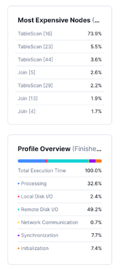
Our query is spending an awful lot of time on TableScan operations.

This means the query spends a lot of time going through the tables in order to find the relevant data. What gives? Our data model is so clean and our query is not very complex.

While you furrow your brow examining these query statistics, your stakeholders come tapping you on the (virtual) shoulder with that familiar look on their face:

Your breathing intensifies. Beads of sweat start rolling down your face. You may be on to something, but we have real users out there with super slow loading reports! Quickly, you huddle with the team and compile a list of potential solutions. You split your team of engineers and divide and conquer:

Simplify Query Complexity

Even though our original query is pretty simple, we can reduce the number columns in our SELECT statement and further refine our WHERE clauses to better leverage our newfound knowledge about micro-partitions. The more we can help the Query Optimizer do its job, the better.

Enable/Disable Query Acceleration Performance

Topic for a future post! In the meantime, have some tasty docs.

Enable/Disable Search Optimization Service

Again, stay tuned! Here's some moar yummy docs.

Split ingestion and querying activities into separate warehouses

Separate the workloads by dedicating distinct Virtual Warehouse instances to ingestion and querying tasks, respectively. Wait, what's a warehouse? Right! Good question. We'll get to this in a minute.

Use Materialized Views as pre-compute for query

We actually did spend some time on this one. While it was a neat experiment and did provide some speedup on the query (since we essentially just pre-computed the data into a giant wide table), it made ingestion, business logic and maintenance unnecessarily complex. Again, stay tuned for more on this in a future post, where we'll be talking materialized views and task graphs!

Increased USER_TASK_MINIMUM_TRIGGER_INTERVAL_IN_SECONDS

Another theory: maybe the ingestion processes are in resource contention with the query processes? If you'll recall, the USER_TASK_MINIMUM_TRIGGER_INTERVAL sets the minimum interval between consecutive task triggers, which prevents the task from executing too frequently. So, if we force a larger pause between task runs, maybe that will leave some breathing room for the queries and reduce resource contention between compute nodes? Sadly, this did not prove to be all that effective.

Added RELY to primary key constraints

What if we reduced redundant joins in our query? Snowflake does not enforce UNIQUE, PRIMARY KEY, and FOREIGN KEY constraints on standard tables.. So, if we're confident in our data model and its inherent relationships between the different tables, we can use the RELY constraint on UNIQUE, PRIMARY KEY, FOREIGN KEY constraints to help the query optimizer eliminate unnecessary joins.

More details here..

Modify or disable clustering

This also made very little difference. But what is clustering? That's what the other half of our team has been working on, so they'll take over from us in a minute!

First things first, let's talk warehouses.

Snowflake Virtual Warehouses Explored

Remember when I talked about Split ingestion and querying activities into separate warehouses ? Yeah, that didn't work. In order to understand why, we need to take a closer look at what a warehouse actually is.

A Snowflake Virtual Warehouse is a cluster of compute resources in Snowflake that processes queries and transactions. Unlike a traditional RDBMS system with static resources, warehouses in Snowflake can be scaled dynamically based on the workload. They provide a completely isolated query execution environment and other features like pausing and auto-suspending of warehouses. This allows Snowflake to do some pretty cool stuff where they can re-use idle resources / nodes / warehouses to buff up compute intensive tasks on other client's warehouses, basically 'borrowing' compute power without charging you, the client, for it. In return, whenever you need a bit of extra juice for a workload, they can do the same for you. What's that? You want docs? Of course, here ya go.

An important consideration when it comes to warehouses is their size, which ranges from XS all the way to 6X-Large as of time of writing.

According to Snowflake:

The size of a warehouse can impact the amount of time required to execute queries submitted to the warehouse, particularly for larger, more complex queries. In general, query performance scales with warehouse size because larger warehouses have more compute resources available to process queries.

If queries processed by a warehouse are running slowly, you can always resize the warehouse to provision more compute resources.

Check out this post to learn more about Snowflake Compute layer and its Virtual Warehouse architecture.

Previously, we used a single XS warehouse for both ingestion and querying workloads. Instead, we decided to:

• Assign an XS warehouse for data ingestion.
• Assign an S warehouse for querying.

Data freshness is not impacted by this split because warehouses are part of the compute layer, which are totally separated from the storage layer. Therefore, data doesn't need to be replicated between warehouses.

The storage layer is fully managed by Snowflake and is built on cloud storage solutions like Amazon S3, Google Cloud Storage or Microsoft Azure Blob Storage. This centralized storage is scalable, secure, and independent of compute resources. In the origin days of Snowflake, they decided to simply offload the storage to cloud vendors so they could specify more on the querying, compute layers and caching layers, which turned out to be a very smart move in the end (no need to build your own data centers if you can rent them for a fraction of the cost, amirite?).

So, in theory, we can add as many warehouses as we want - they would all have instant access to the same data. We (as the client) just tell Snowflake which cloud provider we want to use and they take care of the provisioning. The data in the respective buckets is usually still their proprietary data format, although they do also support open-source formats like Parquet, Avro, XML, etc...

So where did the warehouse resizing leave us?

In theory, moar compute power == faster queries, right? After all, that's what the docs tell us. WRONG. Increasing the warehouse size did not improve query latency.

As it turns out, we missed a critical detail that tells us whether or not it was the available compute resources being the bottleneck for our query speed: If the warehouse does not have enough remaining resources to process a query, the query is queued, pending resources that become available as other running queries complete.

Snowflake provides insight into this via its INFORMATION_SCHEMA.QUERY_HISTORY, which shows query queuing statistics.

A more holistic overview can also be seen in the Warehouses section of the SnowSight Admin UI.

!Warehouse Overview

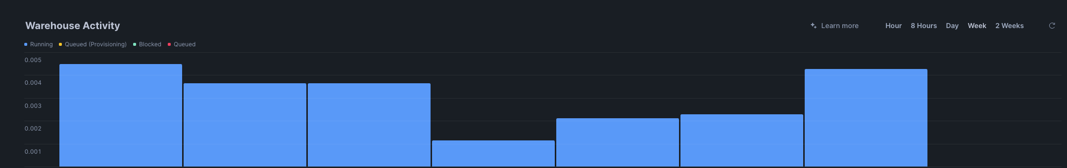
Over the past two weeks, there were no queued queries. So, this means compute resources were sufficient after all?

Sigh...back to the drawing board we go.

So, resizing the warehouse didn’t exactly do what we hoped. The query latency didn’t budge, and it turns out compute resources weren’t the issue after all. With no queries getting stuck in a queue, we know it’s something else. What’s actually slowing things down? It might be time to take a closer look at the way our data is organized. In part 2 of this series, we’ll dive into clustering and partitioning to see if they hold the key to fixing this. See you there!